Last Updated on April 28, 2026 by Vivekanand
In Part 6 of this series, we watched the compiler’s register allocator solve one of the hardest problems in the backend — mapping thousands of virtual registers onto a handful of physical ones. The result is a fully realized object file: machine instructions with physical register assignments, stack frame layouts, and concrete encodings. But these linker object files are not yet executable. They contain code that references functions and global variables whose final addresses are unknown. The linker is the program that resolves these mysteries.
If you have read our Assembly series, you have already seen linking from the runtime side — Part 6 covered the GOT, PLT, and lazy binding that the dynamic linker performs at execution time. This post takes the complementary perspective: what happens at build time, before your program ever runs. We will trace how the static linker reads linker object files, resolves symbols, patches addresses, and produces the final executable that your operating system loads into memory.
Table of Contents
1. Understanding Linker Object Files — What Happens After Compilation
When you compile a multi-file C program, each source file is compiled independently into an object file (.o on Linux/macOS, .obj on Windows). As we traced in Part 1 of this series, the compilation pipeline runs preprocessing, parsing, optimization, and code generation — all per file. The linker is the final stage that stitches these independent pieces together.
The linker performs three core tasks with linker object files. First, symbol resolution: matching every function call and variable reference to its actual definition, even when that definition lives in a different object file or library. Second, relocation: patching placeholder addresses in the machine code with the real, final addresses computed during linking. Third, section merging: combining the .text, .data, .rodata, and .bss sections from every input object file into single unified sections in the output executable.
Section Merging — Building the Final Layout
Each object file has its own set of sections — its own .text (code), .data (initialized globals), .rodata (constants), and .bss (zero-initialized globals). If you recall from Assembly Part 4: Executable Formats, the final ELF or PE executable also has these sections — but only one of each. The linker concatenates all same-named sections together:
  math.o              utils.o             main.o
┌───────────┐    ┌───────────┐     ┌───────────┐
│  .text    │    │  .text    │     │  .text    │
│ (add,mul) │    │ (print)   │     │  (main)   │
├───────────┤    ├───────────┤     ├───────────┤
│  .data    │    │  .data    │     │  .data    │
│ (counter) │    │ (buffer)  │     │ (config)  │
├───────────┤    ├───────────┤     ├───────────┤
│  .rodata  │    │  .rodata  │     │  .rodata  │
│ ("hello") │    │ ("%d\n")  │     │ ("done")  │
└───────────┘    └───────────┘     └───────────┘
        │               │                │
        └───────────┬───┘────────────────┘
                    ▼
            Final Executable
        ┌─────────────────────┐
        │      .text          │
        │ add, mul, print,    │
        │ main (concatenated) │
        ├─────────────────────┤
        │      .data          │
        │ counter, buffer,    │
        │ config              │
        ├─────────────────────┤
        │      .rodata        │
        │ "hello", "%d\n",    │
        │ "done"              │
        └─────────────────────┘
Once sections are merged, every function and variable has a known offset within the final executable. This is when the linker can compute absolute addresses and patch the relocation entries — the placeholder addresses the compiler left behind.
2. Symbol Tables — The Linker’s Roadmap
Every object file contains a symbol table — a directory of all functions and global variables defined or referenced in that file. The linker reads these tables to build a global map of the entire program. You can inspect an object file’s symbol table using nm or readelf -s.
Consider a simple two-file program. File math.c defines add and multiply; file main.c calls them. After compiling each file to an object file with gcc -c, running nm reveals exactly what the linker sees:
$ nm math.o
0000000000000000 T add
0000000000000014 T multiply

$ nm main.o
                 U add
                 U multiply
0000000000000000 T main
                 U printf
The T flag means the symbol is defined in the text (code) section — these are the actual function implementations. The U flag means undefined — main.o references add, multiply, and printf, but does not contain their code. The linker’s job is to match every U with a corresponding T (or D for data, B for BSS). If any symbol remains unresolved after scanning all input files and libraries, you get the dreaded undefined reference to 'function_name' error.
Strong vs Weak Symbols
Not all symbols are equal. By default, function and initialized variable definitions are strong symbols — the linker will reject multiple definitions of the same strong symbol across different linker object files. This is the “multiple definition of” error. Uninitialized global variables and symbols explicitly marked with __attribute__((weak)) are weak symbols. When a strong and weak symbol share the same name, the linker picks the strong one. When multiple weak symbols conflict, the linker picks one arbitrarily. This mechanism is how C libraries provide default implementations that programs can override — a pattern used extensively in embedded systems and plugin architectures.
For a deeper look at how these symbols ultimately end up in the ELF header’s symbol table that the dynamic linker and OS loader read, see Assembly Part 5: Process Loading.
3. Relocation Records — How Addresses Get Patched
When the compiler generates machine code, it does not know where functions or global variables will end up in the final binary. It cannot hard-code the address of add() into a call instruction because the linker decides the final layout. Instead, the compiler emits a relocation record — a note that says “at offset X in this section, insert the address of symbol Y.”
You can see these records with readelf -r:
$ readelf -r main.o

Relocation section '.rela.text' at offset 0x1d8 contains 3 entries:
  Offset          Info           Type                Sym. Value    Sym. Name + Addend
000000000009  000a00000004 R_X86_64_PLT32    0000000000000000 add - 4
000000000018  000b00000004 R_X86_64_PLT32    0000000000000000 multiply - 4
000000000027  000c00000004 R_X86_64_PLT32    0000000000000000 printf - 4
Each entry tells the linker: at the specified Offset in the .text section, patch in the address of the named symbol. The Type field specifies how to compute the address. R_X86_64_PLT32 means “compute a 32-bit PC-relative offset to the symbol’s PLT entry (or direct address for static linking).” The - 4 addend accounts for the fact that x86-64 call instructions compute the relative offset from the end of the instruction, not the beginning.
Walking Through a Relocation
Let’s trace exactly what happens. When the compiler emits a call add instruction in main.o, the machine code looks like this before linking:
Before linking (main.o):
  0x08:  e8 00 00 00 00      call 0x0     ← placeholder (offset = 0)

After linking (executable):
  0x401028:  e8 d3 ff ff ff   call 0x401000  ← patched with real offset to add()
The e8 byte is the x86-64 opcode for a near call with a 32-bit relative displacement. Before linking, the four displacement bytes are all zeros — a placeholder. The linker knows that add() was placed at 0x401000 and the call instruction lives at 0x401028. The relative offset is 0x401000 - (0x401028 + 5) = -0x2d which is 0xffffffd3 in two’s complement. The linker writes those bytes into the instruction, and the call now jumps to the correct address.
This is the same relocation machinery that feeds into the GOT and PLT for dynamic linking at runtime, which we explored in detail in Assembly Part 6: Dynamic Linking. The difference is timing: the static linker patches addresses at build time, while the dynamic linker patches them at load time or on first call.
4. Static vs Dynamic Linking — The Full Comparison
With the mechanics of linker object files understood, we can now examine the two fundamental linking strategies and their trade-offs.
In static linking (gcc -static), the linker copies all required code from object files and static libraries (.a archives) directly into the final executable. Every function your program calls — including C library functions like printf — is physically embedded in the binary. The result is a standalone executable with zero runtime dependencies.
In dynamic linking (the default), the linker only records which shared libraries (.so / .dylib / .dll) are needed. The actual code remains in separate library files, and the dynamic linker (ld-linux.so) loads them into memory at runtime. Function calls go through the PLT/GOT indirection we covered in Assembly Part 6.
| Feature | Static Linking | Dynamic Linking |
|---|---|---|
| Binary Size | Large (includes all library code) | Small (references external libs) |
| Runtime Dependencies | None — fully self-contained | Requires shared libraries present |
| Startup Time | Faster (no runtime symbol resolution) | Slightly slower (PLT/GOT setup) |
| Memory Sharing | No sharing — each process has its own copy | Shared libraries mapped once, shared across processes |
| Security Updates | Must recompile to pick up library fixes | Update the .so file — all programs benefit |
| Call Overhead | Direct call (no indirection) | Indirect via PLT stub + GOT entry |
| Distribution | Easy — single binary, no “DLL hell” | Must ensure correct library versions |
Seeing the Difference in Assembly
The distinction is visible at the assembly level. When you compile with -fPIC (Position-Independent Code, required for shared libraries), external function calls go through PLT stubs. Without -fPIC, the compiler can emit direct calls that the static linker patches directly. Compare these two patterns:
# With -fPIC (dynamic linking target):
call   compute@PLT          # indirect via Procedure Linkage Table

# Without -fPIC (static linking target):
call   compute              # direct call, linker patches address
The @PLT suffix tells the assembler to generate a relocation that routes through the PLT stub. Each PLT entry is a small trampoline that jumps through the GOT — a table of function pointers that the dynamic linker fills in at runtime. This double indirection costs a few extra cycles per call, but it enables the shared library model that modern operating systems depend on.
Interactive: x86-64: Static Call vs PLT Call Comparison on Godbolt
5. Link-Time Optimization — When the Compiler Takes Over Linking
Traditional compilation has a fundamental limitation: each source file is optimized in isolation. The compiler sees only one translation unit at a time, so it cannot inline a function defined in math.c into a call site in main.c. It cannot eliminate a global variable that is written in one file but never read anywhere in the entire program. The boundary between translation units is an optimization wall.
Link-Time Optimization (LTO) demolishes this wall. When you compile with -flto, the compiler does not produce machine code in linker object files. Instead, it embeds LLVM IR (or GCC’s GIMPLE IR) in the object files. At link time, the linker hands this IR back to the compiler, which now sees the entire program at once — every function, every variable, every call site. It can then apply all the optimization passes we covered in Part 4: Optimization Passes across module boundaries.
The impact is dramatic. Consider two files:
// math.c
int square(int x) {
    return x * x;
}

// main.c
extern int square(int x);

int process(int a) {
    return square(a) + square(a + 1);
}
Without LTO, the compiler cannot inline square() into process() because they are in different files. The generated assembly contains two call square instructions with full calling convention overhead — saving registers, setting up arguments, restoring state. With -flto -O2, the linker-integrated optimizer sees both functions simultaneously. It inlines square(), eliminates the function call overhead entirely, and produces tight arithmetic that never touches the stack:
# Without LTO: two function calls
process:
    push   rbx
    push   r14              # save callee-saved registers
    mov    ebx, edi
    call   square           # first call — ABI overhead
    mov    r14d, eax
    lea    edi, [rbx + 1]
    call   square           # second call — ABI overhead
    add    eax, r14d
    pop    r14
    pop    rbx
    ret

# With -flto -O2: everything inlined
process:
    mov    eax, edi
    imul   eax, edi         # x * x inlined
    lea    ecx, [rdi + 1]
    imul   ecx, ecx         # (x+1) * (x+1) inlined
    add    eax, ecx
    ret                     # no calls, no stack frame
LTO also enables cross-module dead code elimination. If a function is defined in utils.c but never called anywhere in the entire program, the linker-integrated optimizer strips it from the final binary. Without LTO, the linker must keep it — it has no way to know if a statically-linked library function might be needed.
Interactive: Cross-Module Inlining: Without LTO vs With -flto on Godbolt
ThinLTO — Scaling LTO to Large Projects
Full LTO loads the entire program’s IR into memory at once, which can consume tens of gigabytes for large codebases like Chrome or the Linux kernel. ThinLTO (-flto=thin in Clang) is a scalable alternative. Instead of merging all IR, it builds a compact summary of each module — function signatures, call graphs, and type information. The linker uses these summaries to make global decisions (what to inline, what to eliminate) but compiles each module’s IR in parallel with only the necessary cross-module information imported. ThinLTO achieves most of Full LTO’s optimization benefits while using significantly less memory and supporting parallel compilation.
6. Linker Scripts — Taking Manual Control
For most application development, the default linker behavior is fine — the linker uses a built-in script that places sections at standard addresses. But when you are writing an operating system kernel, a bootloader, or bare-metal firmware, you need precise control over where every section lands in memory. This is where linker scripts come in.
A linker script tells the linker exactly how to arrange linker object files‘ sections in the output. Here is a minimal example for a bare-metal ARM Cortex-M program:
/* minimal.ld — Bare-metal linker script */
ENTRY(_start)

MEMORY {
    FLASH (rx)  : ORIGIN = 0x08000000, LENGTH = 256K
    SRAM  (rwx) : ORIGIN = 0x20000000, LENGTH = 64K
}

SECTIONS {
    .text : {
        *(.vectors)     /* Interrupt vector table first */
        *(.text*)       /* All code sections */
        *(.rodata*)     /* Read-only data with code */
    } > FLASH

    .data : {
        *(.data*)       /* Initialized variables */
    } > SRAM AT > FLASH  /* Runs from SRAM, stored in FLASH */

    .bss : {
        *(.bss*)        /* Zero-initialized variables */
    } > SRAM
}
The MEMORY block defines the physical memory regions — flash ROM at 0x08000000 and SRAM at 0x20000000. The SECTIONS block maps each input section type to a specific memory region. The > FLASH directive tells the linker to place .text in flash. The > SRAM AT > FLASH for .data means the initialized data is loaded from flash but runs from SRAM — the startup code (_start) must copy it before main() runs.
The Linux kernel uses elaborate linker scripts to control its memory layout — placing the interrupt vector table at a fixed address, aligning page tables to 4KB boundaries, and creating special sections for kernel modules that can be loaded and unloaded. You can view the kernel’s linker script at arch/x86/kernel/vmlinux.lds.S in the Linux source tree. For the complete linker script syntax, see the GNU ld documentation.
7. Conclusion
The linker is often the least understood part of the compilation pipeline, yet it is the program that makes multi-file projects possible. It reads the linker object files produced by the compiler backend, resolves every symbol reference into a concrete address, patches machine code through relocation records, and merges sections into the final executable layout. Without it, every C program would have to live in a single source file.
We have also seen how Link-Time Optimization blurs the boundary between compilation and linking — handing the linker IR instead of machine code enables cross-module optimizations that are impossible when each file is compiled in isolation. And for embedded and kernel development, linker scripts provide the surgical control over memory layout that those environments demand.
With this post, we have traced the complete journey from C source code to executable binary — from Part 1’s pipeline overview through lexing, parsing, IR, optimization, code generation, register allocation, and now linking. The compiler pipeline is no longer a black box. In Part 8: Writing a Toy Compiler from Scratch, we will put everything into practice by building a working compiler from the ground up — a lexer, parser, and code generator that takes a simple language and produces real x86-64 assembly. We will need every concept from this series.